Overview

Feel free dive straight into the simulation via the simulation Tab.

The tech stack is self-hosted on an NVIDIA Jetson, as the original goal of the project was to achieve a real-time simulation capable of running on a vehicle. The simulation is developed in C++, with keyframe data passed to a Python Flask server via shared memory, utilizing the multiprocessing.shared_memory module introduced in Python 3.8. This approach significantly reduces overhead compared to traditional input/output methods by enabling efficient, memory-mapped data exchange between prgrams. Flask processes this data into JSON format, which is then transmitted to the JavaScript front end powered by Three.js for 3D visualization. Additionally, graphs displaying simulation data are dynamically compiled from the same keyframe JSON using Plotly.js.

On the current ARM processor from 2017, the simulation calculates a 3-minute scenario with a static timestep of 0.01 seconds per step—approximately 18,000 steps—in just 1.5 to 1.8 seconds. This computation time includes a significant number of steps that are discarded due to prediction vehicles being cast to evaluate the consequences in the future(over the horizon). The fast computation speed provides flexibility for error correction, allowing the system to proactively prevent future unwanted states based on these predictions.

Physics Engine

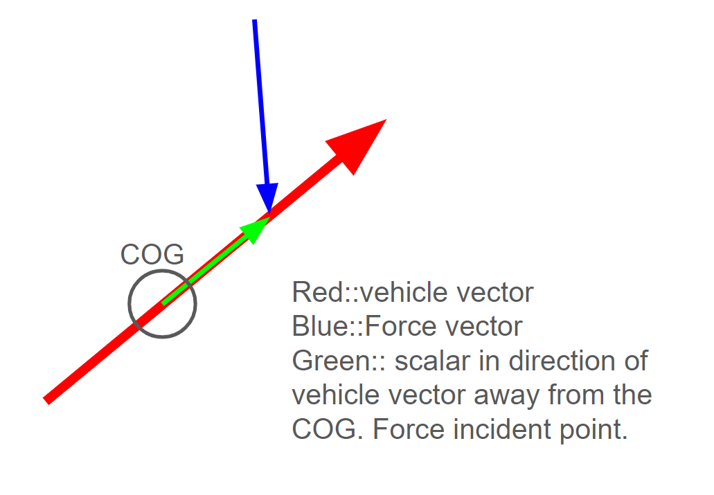
The vector representation shown in Figure 1 serves as the basis for the forces acting on the vehicle body. To fully determine the outcome of a force acting on the body, both linear acceleration and moments must be calculated. In Euclidean space, the simulation can be interpreted along three independent axes. First, the summation of all forces is computed to obtain a resultant force vector. This force is then applied to the body of the vehicle using the following series of equations.

Using the change in velocity and the velocity vector of the previous timestep(n - 1), we can easily compute the next state.

Extending to a change in position.

Rotation matrices are used to manipulate vectors and update the vehicle's orientation in 3D space. The following matrices can rotate a vector around the axis defined.

Multiplying the matrices returns a resultant matrix that can rotate a vector in 𝑅³.

A potential improvement to the simulation could be the use of quaternions instead of rotation matrices for handling rotations. Quaternions offer better stability when dealing with floating-point errors, which can cause numerical instability in rotation matrices. They also avoid issues like gimbal lock and require less memory and computation. This could result in more efficient and accurate simulations of continuous rotations in 3D space, enhancing both performance and precision.

The simulation uses a Runge kutta method called RK4. Rk4 uses a weighted average of a defined set of discretized points to increase the precision of Euler's method. The image in figure x shows the increase in precision over an example differential equation.

For the differential equation \( \frac{dy}{dt}\) = f(t,y) , where \( \frac{dy}{dt}\) is a function of t and y. The weighted average is defined by the following.

y_n+1 is the estimation of the next step using the previous step y_n as a foundation.

Aerodynamic Interpolation

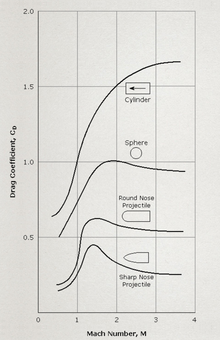
The aero model is a combination of two orthogonal vectors, lift and drag. The drag vector is antiparallel to the airstream relative to the vehicle. A rocket creates lift by using its body as a “lifting body”. The coefficient of lift is directly related to the angle of attack relative to the oncoming air. Although the body is cylindrical and doesn't have wings, the small coefficient of lift at high velocity makes the vehicle maneuverable. In the current state the cross sectional area and coefficient of drag and lift are crudely estimated. Both are augmentations from a circular cross section to a rectangular cross section. The image in figure 4 shows the drag coefficient for a square ended cylinder given a mach number.

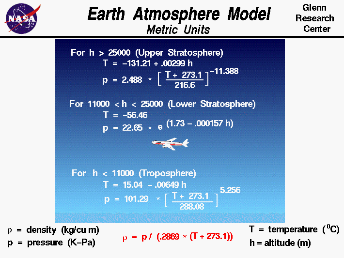
To accurately estimate the vehicle's reentry, air density is a crucial variable. Using the vehicle's Z position and the chart in the figure . The stepwise functions were tested via an empirical lookup table. Much of the behavior in high altitude tests can be attributed to the variability of air densities well entering the atmosphere.

Reentry Burn

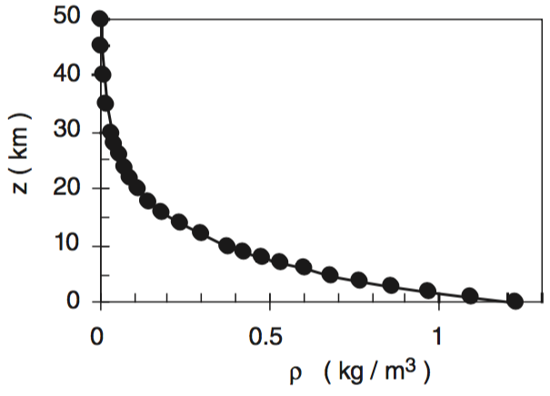
The Falcon 9 entry burn is a strategic propulsive maneuver that reduces velocity, controls descent trajectory, and manages energy dissipation during atmospheric reentry, enabling precise and recoverable rocket landing. A large reduction in velocity is required prior to hitting a wall of air. Air density increases exponentially as the vehicle decreases in altitude. The graph in Figure 5 shows this relationship between altitude and air density.

A vehicle traveling at 2000 m/s tangentially to the atmosphere in a suborbital trajectory, more than 100 km above the Earth, will decelerate at a rate exceeding 90 m/s². The burn also reduces the amount of heat generated from aerodynamic drag/friction. If we assume that all drag is converted to heat energy (likely a poor assumption, but it helps paint a picture), we can use the following equations to see the relationship between vehicle velocity and heat generation.

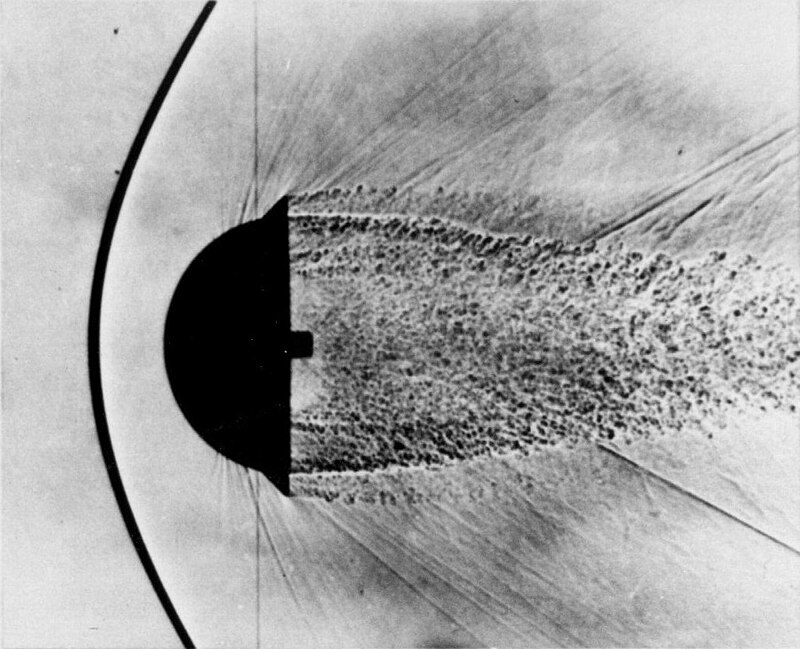
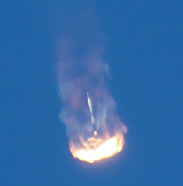
Another adverse effect of the reentry burn might be the increase of pressure at the engines of the vehicle. This pressure is called ram pressure, and it’s used in the blunt bodies of reentry spacecraft. The blunt body creates a boundary layer of air that pushes the heated shock layer forward (away from the vehicle). The pictures in figure 6 and 7 show the resemblance of the shock wave. This is speculative, as a more in-depth finite element or particle simulation would be needed to analyze low-level fluid dynamics.

Landing Burn

The landing control is currently being done with a feedforward control loop. Feedforward control anticipates the required control output based on the system's current state and desired outcome, rather than reacting to errors. A combination of feedforward and feedback control loops allow us to preemptively anticipate system variables while reacting to errors. A graphical representation is shown in figure 4. The simulation is using PID as a feedback controller. The feedforward controller uses the required force to determine the angle of attack(AOT) of the vehicle.

In an ideal scenario, the horizontal and vertical velocities would come to rest simultaneously when the vehicle reaches a Z position of zero. Over the small time-step interval of the simulation, a linear acceleration assumption can be made. The deceleration of the X, Y, and Z components can be synchronized. First, the simulation calculates the required deceleration rate.

Using the time required to decelerate the Z-axis velocity to zero, the X and Y accelerations can be interpolated.

As time to impact approaches 0, the feedforward calculation begins to break down. As the vehicle approaches landing, the control requests become erratic due to the rapid growth in the request acceleration.

Using the Acceleration the force request can be calculated.

Before the vehicle can begin to decelerate, a desired angle of attack (AOT) must be achieved. The desired AOT is represented as a vector that defines the target vehicle state, independent of its location. Using a series of control loops—each managing the engine gimbal angle, vehicle orientation, and thrust force—the vehicle can effectively reduce its sideslip velocity.

The ideal thrust force application is such that no additional parasitic moment is created. An off axis thrust force would inherently cause a vehicle moment.Therefore, the ideal angle of attack aligns with the antiparallel axis of the thrust force. The angle of attack can be defined as follows.

A potential improvement to this control stack would be to implement a feedforward version of the vehicle angle control loop. Currently, thrust is not integrated into the loop, meaning the gains of the rotation control loop are not scaled according to the engine's output power. The control loop should be linked to a moment request, as defined by the equation below.

In other words a small amount of thrust would demand a large gimbal movement. Conversely, a large thrust vector would demand a small movement. The current control loop is being corrected via the error in euler angles when comparing the vehicle vector and the angle of attack vector.

Preset Simulation Parameters